
ParkSEIS© (PS) -
Passive MASW (Data Acquisition and Processing)
The most common purpose for running a passive MASW survey is to increase the investigation depth (Zmax) beyond the limit of most active surveys
(e.g., 30 m). There are two conditions that have to be met to increase Zmax; a more powerful source that can generate "strong" low frequencies
(long wave-lengths) of surface waves, and a longer receiver array that can effectively record such long wavelengths.
The impact power (E) of an active source like a sledge hammer can be increased by adding more weight (m) and/or increasing the impact speed (v)
because it is the kinetic energy [E = (1/2)mv2] that is transformed into the elastic (seismic) energy upon impact. In this way, an accelerated weight
drop source can generate a greater E than a sledge hammer. In reality, however, this artificial increase of E can be limited because it eventually
faces the obstacle of operational and economical cost. That's why the passive MASW surveys utilizing ambient vibrations (usually generated from
traffic) have become popular. Figure 1 illustrates the comparison of E from typical active and passive sources. It indicates the common passive E is
greater than the active E by a few orders of magnitude. These surface waves from of traffic origin are generated from irregular places on the road
when vehicles are travelling over them (Figure 2). The usual frequency range is from a few to a few tens of hertz (e.g., 1-30 Hz) and the low-end
frequencies (e.g., 1-10 Hz) are most useful because they are not easily generated with sufficient energy using typical active sources, but are often
critical to increase Zmax beyond the common range (e.g., ≥ 30 m). It is speculated that the combination of the large mass and shock-absorbing
mechanism (tire and suspension spring) of the vehicle facilitates the generation of such low frequency surface waves.
The array length (L) has to be in proportion to the Zmax; the longer array is needed for a deeper investigation. The most commonly used
relationship between the two is KminL ≤ Zmax ≤ KmaxL, with Kmin = 0.5 and Kmax = 1.0. Although the actual relationship can be influenced by
other acquisition and processing factors such as signal-to-noise (SN) ratio of acquired data and the specific algorithm used during the dispersion
analysis, the most common rule of thumb is L = 2Zmax (Figure 3). In this case, it is usually assumed that the optimum source offset (X1) is about
1/4 of the array length; i.e., X1 = (1/4)L (Park et al., 1999; Park et al., 2002; Park and Carnevale, 2010). It is also the source offset (X1) that can
contribute positively in increasing Zmax (Park and Carnevale, 2010; Yoon and Rix, 2009). Therefore, some studies indicate it should be X1 + L =
2Zmax (Yoon and Rix, 2009). In this case, X1 should remain within a reasonable range to avoid the use of an excessively short (or long) array; for
example, X1 + L = 2Zmax with X1 ≤ L. However, it seems that the significance of X1 can vary with site geology (i.e., velocity structure) and it can be
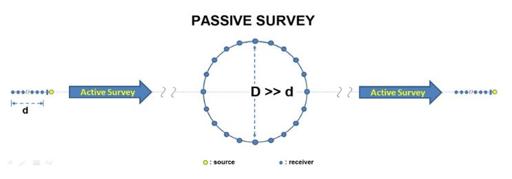
out of the equation as far as the array length (L) becomes sufficiently long for Zmax (for example, L ≥ 2Zmax). With a passive survey, the dimension
(D) of the array is set approximately twice Zmax (Figure 4); D ≈ 2Zmax. This also applies to the active/passive combined survey that is essentially
identical to the active survey using a long recording time (e.g., T ≥ 30 sec) as further explained below.
Although it is always recommended to use a 2-D array for a passive survey such as a circle or an L-shaped array for the maximized accuracy in
dispersion analysis, it is not always convenient to secure such spacious areas, especially during an urban survey. Deployment of the conventional
linear (1-D) array is often the only option available. The most convenient way of utilizing passive surface waves during an active survey for the 2-D
velocity (Vs) profiling is the active/passive combined survey. This is the same as an ordinary active survey that uses the linear array and continues to
make measurements at successive locations by moving the source/receiver configuration (i.e., a roll-along survey). The only difference is its
recording time (e.g., T ≥ 30-sec) significantly longer than the usual time used in an active survey (e.g., T=2-sec). The first 1-2 seconds of the record
will contain most of the active surface waves, while the rest of the record contains ambient vibrations of passive surface waves. In this way, it is a
combination of the conventional active survey and the passive survey using the 1-D (linear) receiver array. Although the dimension of the passive
array in this case (i.e., D=L) will be shorter than the length usually recommended for a passive survey (e.g., D≈2L), the recorded strong low-
frequency surface waves will increase the chance of imaging dispersion patterns at the lowest frequencies with the highest definition that the given
array can ever provide. This is the way the investigation depth can exceed the range that can be achieved by an active survey alone; for example,
Zmax ≥ L.
A passive MASW can be executed during either 1-D or 2-D velocity (Vs) profiling for the purpose of an increased investigation depth (Zmax). During
the survey for 1-D Vs profiling, the separate active survey has to be performed near the center of the array used for the passive survey. The field
geometry for the active survey can be chosen in such a way that it can cover depths about half the Zmax aimed for during the passive survey. During
the survey for 2-D velocity (Vs) profiling, the passive survey can be arranged at one location (e.g., at the center of the survey line) or multiple locations
(e.g., at the beginning, the center, and the end of the survey line) with a dimension (D) of D ≥ 2L as illustrated in Figure 5.
There are two ways to utilize passive MASW data (Figure 6)—providing the fundamental-mode (M0) dispersion at such low frequencies where the
active data usually fails to show any meaningful patterns (Figure 6a); and providing dispersion patterns that, when combined with patterns analyzed
from the active data, can make the overall modal interpretation more effective (Figure 6b). In any case, the passive data is not used by itself and
always used in combination with active data. The former way of utilization is most common because it directly leads to an increased Zmax. The
latter is chosen when it is necessary to accurately interpret those complicated dispersion patterns otherwise interpreted erroneously or that are
difficult to interpret at all. The more accurate dispersion analysis facilitated in this way will result in the more accurate velocity (Vs) profile at the end.
This type of utilization, however, requires a systematic preparation of data acquisition and processing steps, and therefore is usually implemented
for research purposes or for certain special projects. The two types of utilization are illustrated in Figure 6 using real field data sets.
In theory, it is the 2-D receiver array (e.g., circle), rather than a 1-D linear array, that can ensure the most accurate dispersion analysis because of the
two unknowns in passive surveys that do not exist in the active surveys—the excitation time and location of the source. The former is not an obstacle
in most data-processing algorithm used nowadays that require only the relative (not absolute) arrival times of surface waves. The source location,
however, is important because it directly influences the phase relationship of surface waves depending on the distance (r) and azimuth (theta) of the
source location. The original formulation of SPAC (spatial autocorrelation) method by Aki (1957) was based on the assumption that recorded
passive surface waves are plane waves generated from an infinite distance (i.e., r >> D) with their azimuths distributed throughout all 360 degrees (i.
e., omni-directional plane waves). This assumption made it possible to cancel out the two variables (r and theta) from the equation through a proper
summation process. The method by Park et al. (2004) also adopted this "omni-directional plane wave" assumption so that it can construct the
dispersion image through the energy summation in r and theta, which in ultimate mathematical formulation can become identical to SPAC. Park
and Miller (2008), however, indicated that those passive surface waves culturally generated (for example, from traffic) rather than naturally generated
(for example, from tidal motion) do not meet the assumption. This research indicated that passive surface waves are often generated from one or a
few irregular surface points on the road near the receiver array so that they usually take the "uni-directional cylindrical" (rather than "omni-directional
planar") propagation. If the dispersion analysis scheme by SPAC or Park et al. (2004) is used in this case, the processed image suffers from a low
definition as well as biased trend of dispersion. In addition, Park (2008) indicated that it is the accurate resolution in azimuth (theta) once the
distance (r) becomes greater than the array dimension (D) that is most critical in constructing an accurate image with the highest definition ever
possible. Park (2010) further improved this concept by dividing a long (e.g., 30-sec) passive record into many subrecords of shorter time (e.g., 2-
sec), each of which is treated as an independent record potentially containing surface waves generated from one (dominating) surface location near
the receiver array (r > D). Therefore, use this method from Park (2010) for dispersion analysis of passive MASW data is highly recommended,
especially when a 2-D receiver array is used. It will provide a useful dispersion image, even when all other methods fail to provide any recognizable
pattern. It can also provide a quality image from the passive data collected by using the 1-D (linear) array. In this case, however, the search for
azimuth (theta) will take place only in forward (theta=0 degree) and reverse (theta=180 degrees) propagations instead of the full 360-degree search.
Park and Miller (2008) indicated that phase velocities can be overestimated if a 1-D array is used during a passive survey.
Passive MASW (Data Acquisition and Processing)
- See user guide.
The most common purpose for running a passive MASW survey is to increase the investigation depth (Zmax) beyond the limit of most active surveys
(e.g., 30 m). There are two conditions that have to be met to increase Zmax; a more powerful source that can generate "strong" low frequencies
(long wave-lengths) of surface waves, and a longer receiver array that can effectively record such long wavelengths.
The impact power (E) of an active source like a sledge hammer can be increased by adding more weight (m) and/or increasing the impact speed (v)
because it is the kinetic energy [E = (1/2)mv2] that is transformed into the elastic (seismic) energy upon impact. In this way, an accelerated weight
drop source can generate a greater E than a sledge hammer. In reality, however, this artificial increase of E can be limited because it eventually
faces the obstacle of operational and economical cost. That's why the passive MASW surveys utilizing ambient vibrations (usually generated from
traffic) have become popular. Figure 1 illustrates the comparison of E from typical active and passive sources. It indicates the common passive E is
greater than the active E by a few orders of magnitude. These surface waves from of traffic origin are generated from irregular places on the road
when vehicles are travelling over them (Figure 2). The usual frequency range is from a few to a few tens of hertz (e.g., 1-30 Hz) and the low-end
frequencies (e.g., 1-10 Hz) are most useful because they are not easily generated with sufficient energy using typical active sources, but are often
critical to increase Zmax beyond the common range (e.g., ≥ 30 m). It is speculated that the combination of the large mass and shock-absorbing
mechanism (tire and suspension spring) of the vehicle facilitates the generation of such low frequency surface waves.
The array length (L) has to be in proportion to the Zmax; the longer array is needed for a deeper investigation. The most commonly used
relationship between the two is KminL ≤ Zmax ≤ KmaxL, with Kmin = 0.5 and Kmax = 1.0. Although the actual relationship can be influenced by
other acquisition and processing factors such as signal-to-noise (SN) ratio of acquired data and the specific algorithm used during the dispersion
analysis, the most common rule of thumb is L = 2Zmax (Figure 3). In this case, it is usually assumed that the optimum source offset (X1) is about
1/4 of the array length; i.e., X1 = (1/4)L (Park et al., 1999; Park et al., 2002; Park and Carnevale, 2010). It is also the source offset (X1) that can
contribute positively in increasing Zmax (Park and Carnevale, 2010; Yoon and Rix, 2009). Therefore, some studies indicate it should be X1 + L =
2Zmax (Yoon and Rix, 2009). In this case, X1 should remain within a reasonable range to avoid the use of an excessively short (or long) array; for
example, X1 + L = 2Zmax with X1 ≤ L. However, it seems that the significance of X1 can vary with site geology (i.e., velocity structure) and it can be
out of the equation as far as the array length (L) becomes sufficiently long for Zmax (for example, L ≥ 2Zmax). With a passive survey, the dimension
(D) of the array is set approximately twice Zmax (Figure 4); D ≈ 2Zmax. This also applies to the active/passive combined survey that is essentially
identical to the active survey using a long recording time (e.g., T ≥ 30 sec) as further explained below.
Although it is always recommended to use a 2-D array for a passive survey such as a circle or an L-shaped array for the maximized accuracy in
dispersion analysis, it is not always convenient to secure such spacious areas, especially during an urban survey. Deployment of the conventional
linear (1-D) array is often the only option available. The most convenient way of utilizing passive surface waves during an active survey for the 2-D
velocity (Vs) profiling is the active/passive combined survey. This is the same as an ordinary active survey that uses the linear array and continues to
make measurements at successive locations by moving the source/receiver configuration (i.e., a roll-along survey). The only difference is its
recording time (e.g., T ≥ 30-sec) significantly longer than the usual time used in an active survey (e.g., T=2-sec). The first 1-2 seconds of the record
will contain most of the active surface waves, while the rest of the record contains ambient vibrations of passive surface waves. In this way, it is a
combination of the conventional active survey and the passive survey using the 1-D (linear) receiver array. Although the dimension of the passive
array in this case (i.e., D=L) will be shorter than the length usually recommended for a passive survey (e.g., D≈2L), the recorded strong low-
frequency surface waves will increase the chance of imaging dispersion patterns at the lowest frequencies with the highest definition that the given
array can ever provide. This is the way the investigation depth can exceed the range that can be achieved by an active survey alone; for example,
Zmax ≥ L.
A passive MASW can be executed during either 1-D or 2-D velocity (Vs) profiling for the purpose of an increased investigation depth (Zmax). During
the survey for 1-D Vs profiling, the separate active survey has to be performed near the center of the array used for the passive survey. The field
geometry for the active survey can be chosen in such a way that it can cover depths about half the Zmax aimed for during the passive survey. During
the survey for 2-D velocity (Vs) profiling, the passive survey can be arranged at one location (e.g., at the center of the survey line) or multiple locations
(e.g., at the beginning, the center, and the end of the survey line) with a dimension (D) of D ≥ 2L as illustrated in Figure 5.
There are two ways to utilize passive MASW data (Figure 6)—providing the fundamental-mode (M0) dispersion at such low frequencies where the
active data usually fails to show any meaningful patterns (Figure 6a); and providing dispersion patterns that, when combined with patterns analyzed
from the active data, can make the overall modal interpretation more effective (Figure 6b). In any case, the passive data is not used by itself and
always used in combination with active data. The former way of utilization is most common because it directly leads to an increased Zmax. The
latter is chosen when it is necessary to accurately interpret those complicated dispersion patterns otherwise interpreted erroneously or that are
difficult to interpret at all. The more accurate dispersion analysis facilitated in this way will result in the more accurate velocity (Vs) profile at the end.
This type of utilization, however, requires a systematic preparation of data acquisition and processing steps, and therefore is usually implemented
for research purposes or for certain special projects. The two types of utilization are illustrated in Figure 6 using real field data sets.
In theory, it is the 2-D receiver array (e.g., circle), rather than a 1-D linear array, that can ensure the most accurate dispersion analysis because of the
two unknowns in passive surveys that do not exist in the active surveys—the excitation time and location of the source. The former is not an obstacle
in most data-processing algorithm used nowadays that require only the relative (not absolute) arrival times of surface waves. The source location,
however, is important because it directly influences the phase relationship of surface waves depending on the distance (r) and azimuth (theta) of the
source location. The original formulation of SPAC (spatial autocorrelation) method by Aki (1957) was based on the assumption that recorded
passive surface waves are plane waves generated from an infinite distance (i.e., r >> D) with their azimuths distributed throughout all 360 degrees (i.
e., omni-directional plane waves). This assumption made it possible to cancel out the two variables (r and theta) from the equation through a proper
summation process. The method by Park et al. (2004) also adopted this "omni-directional plane wave" assumption so that it can construct the
dispersion image through the energy summation in r and theta, which in ultimate mathematical formulation can become identical to SPAC. Park
and Miller (2008), however, indicated that those passive surface waves culturally generated (for example, from traffic) rather than naturally generated
(for example, from tidal motion) do not meet the assumption. This research indicated that passive surface waves are often generated from one or a
few irregular surface points on the road near the receiver array so that they usually take the "uni-directional cylindrical" (rather than "omni-directional
planar") propagation. If the dispersion analysis scheme by SPAC or Park et al. (2004) is used in this case, the processed image suffers from a low
definition as well as biased trend of dispersion. In addition, Park (2008) indicated that it is the accurate resolution in azimuth (theta) once the
distance (r) becomes greater than the array dimension (D) that is most critical in constructing an accurate image with the highest definition ever
possible. Park (2010) further improved this concept by dividing a long (e.g., 30-sec) passive record into many subrecords of shorter time (e.g., 2-
sec), each of which is treated as an independent record potentially containing surface waves generated from one (dominating) surface location near
the receiver array (r > D). Therefore, use this method from Park (2010) for dispersion analysis of passive MASW data is highly recommended,
especially when a 2-D receiver array is used. It will provide a useful dispersion image, even when all other methods fail to provide any recognizable
pattern. It can also provide a quality image from the passive data collected by using the 1-D (linear) array. In this case, however, the search for
azimuth (theta) will take place only in forward (theta=0 degree) and reverse (theta=180 degrees) propagations instead of the full 360-degree search.
Park and Miller (2008) indicated that phase velocities can be overestimated if a 1-D array is used during a passive survey.
| |
| |
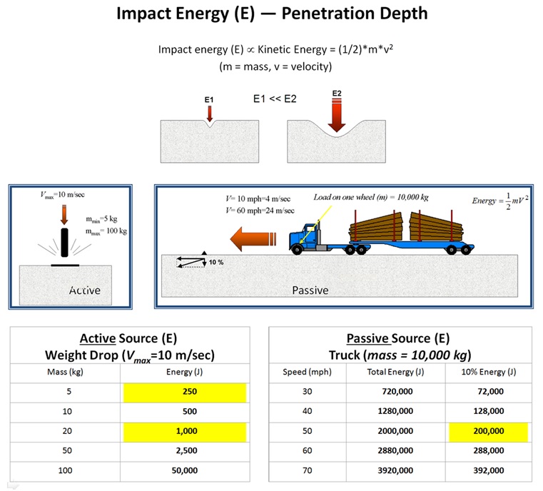
- Figure 1. Comparison of impact energy from typical active and passive sources.
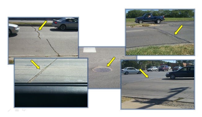
- Figure 2. Irregular road surfaces that generate surface waves when vehicles are moving over them.
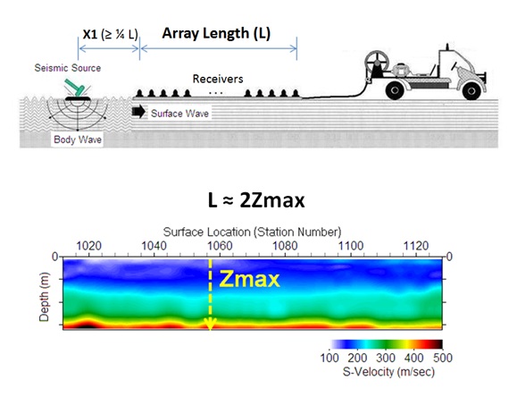
- Figure 3. Relationship between the receiver array length (L) and maximum investigation depth
(Zmax) used during an active survey.
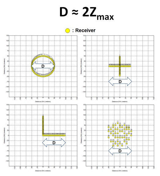
- Figure 4. Relationship between the receiver array dimension (D) and maximum investigation depth
(Zmax) used during a passive survey.
- Figure 5. Illustration showing that the passive survey with a 2-D receiver array may be most optimally executed at a place
near the center of an active survey line.
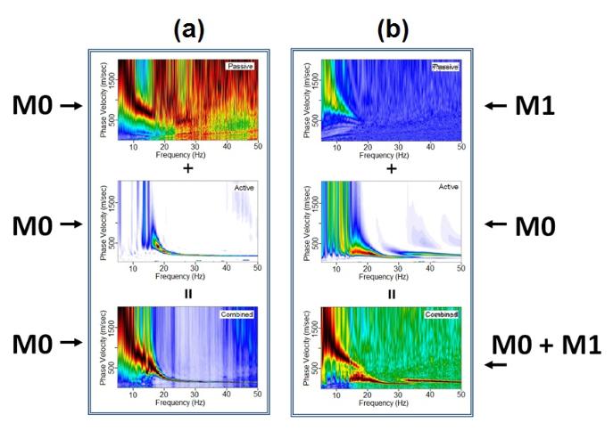
- Figure 6. Two possible ways of utilizing the passive dispersion image. The first (a) provides the trend of fundamental-
mode (M0) dispersion at the lower frequencies; the second (b) provides a constraint for more accurate modal
interpretation of observed dispersion trends.
Park Seismic LLC, Shelton, Connecticut, Tel: 347-860-1223, Fax: 203-513-2056, Email: parkseis@parkseismic.com
