
ParkSEIS© (PS) -
Back Scattering Analysis (BSA) and Common-Offset Sections
The most common output of a 2-D shear-wave velocity (Vs) cross section shows only a general velocity (Vs) variation trend that often may not have
sufficient resolution to detect small-scale anomalies such as underground utility pipes and tunnels. This is because MASW is not an imaging
method that is based on the focusing principle (Claerbout, 1985) (Figure 1). The approach for normal MASW analysis is based on the layered-earth
surface-wave propagation in which only the vertical variation is considered. Therefore, the solution of the individual 1-D (depth) velocity (Vs) profile
obtained from each field record represents the "best" vertical velocity (Vs) model by laterally averaging subsurface properties under the receiver array
used to acquire the record. In this case, an anomaly whose size (D) is smaller than a few receiver spacings (dx) (e.g., D ≤ 2dx for 24-channel
acquisition) may not be able to make a significant impact on the dispersion property of surface waves. As a consequence, the 2-D velocity (Vs)
cross section may not be the optimal approach to detect anomalies. On the other hand, a small object can generate strong back-scattered surface
waves that can be visually identified sometimes over many receiver stations in the field records (Figure 2).
Horizontally travelling surface waves impinging into an object are scattered into all directions as if the object is a new source point (Huygen's
Principle). Those travelling backward along the receiver line are called back-scattered surface waves (Figure 3), which make a distinctive arrival
pattern of opposing slope in comparison to those of forward propagation travelling directly from the source (Figure 2). By observing the surface
location where the feature originates, the anomaly is detected in its horizontal coordinate (Figures 2 and 3). Although the back-scattering does not
noticeably influence dispersion analysis that focuses only to the forward propagation, the feature itself can be used to detect anomalies. In this
case, the horizontal accuracy can be as high as one receiver spacing (1dx), although the vertical (depth) accuracy may be less (Figure 4).
The minimum dimension of an object to be detected by body (reflected) wave is ultimately determined by wavelength of the impinging wave. A
shorter wavelength will be needed to detect a smaller object. The same principle must apply to the back scattering of surface waves. In surface
waves, however, penetration depth (Zp) is in proportion to wavelength of surface waves (Lamda); the longer wavelength penetrates deeper. In
general, one wavelength is considered the penetration depth (Zp ≈ 1Lamda) as most of the surface wave energy (≥ 99%) is confined for depths
shallower than that (Richart et al., 1970) (Figure 5). Then, the minimum size of the (void) anomaly (Dmin) that can be detected by back scattering
becomes a function of its depth of existence (Za); Dmin ≈ kZa with (k < 0.5). Although no such theoretical studies have been reported, observations
made based on the real and numerical experiments indicate that it is a small fraction of Za; for example, Dmin ≈ 0.2Za. This relationship accounts
for not only the wavelength-dependent aspect of detectability but also the amplitude (A) of surface wave that decreases exponentially with depth (Z)
(Sheriff and Geldart, 1985); i.e., A ≈ exp (-aZ) with a > 0.0.
The approximate depth of the anomaly can be depicted from the spectral characteristics of the back-scattering feature by utilizing the wavelength
(Lamda) dependent penetration depth (Zp) of surface waves (Zp ≈ Lamda). The back scattering can occur only when Zp exceeds the top of the
anomaly of size D existing at depth Za (Figure 5); i.e., Zp > Za-D/2. Depending on the spectral characteristics of impinging surface waves and also
on the ambient noise characteristics, the wavelength that gives the strongest back scattering may change. There are no systematic studies reported
that address this subject through theoretical analysis. However, empirical observations indicate that an approximate relationship should follow the
trend illustrated in Figure 6. It shows that, for a given size D (≈ 0.2Za), the back scattering amplitude increases with wavelength once it penetrates
deeper than top of the anomaly (i.e., Zp ≈ Lamda > Za-D/2), and the maximum amplitude occurs when Zp ≈ Lamda ≈ 2Za (Figure 6). Then, the
amplitude gradually decreases as Zp (or Lamda) further increases. The specific shape of the curve illustrated in Figure 6 and the wavelength that
gives the strongest back scattering (i.e., Lamda ≈ 2Za) should change to a certain extent depending on the size (D) of the anomaly as well as the
spectral characteristics of impinging surface waves.
The relationship of Zp ≈ Lamda ≈ 2Za that gives the strongest back scattering provides a way of approximately evaluating the depth of anomaly (Za)
that is responsible for the observed back-scattering feature. For example, if its dominant frequency is observed as fa and the corresponding phase
velocity in the measured dispersion curve is Cf, then its depth is calculated as Za ≈ (1/2) Lamda = (1/2)(Cf/fa). Therefore, if
fa = 20 Hz and Cf = 160 m/sec, then Za ≈ 4 m. This is an approximate evaluation of the depth to the (vertical) center of the anomaly. Depth to the top
of the anomaly (ZT) can usually be estimated more accurately than Za through successive narrow-band-pass (NBP) filtering. For example, if the
back-scattering feature completely disappears after a NBP filtering with pass-band parameters of 45 Hz-50Hz -50 Hz-55 Hz (i.e., NBP filtering
centered at 50 Hz) has been applied and Cf = 150 m/sec at 50 Hz (from measured dispersion curve), then ZT > 3 m (i.e., top of the anomaly is
deeper than 3 m).
The back-scattering analysis (BSA) algorithm incorporated in this software tries to enhance those back-scattered surface waves as much as
possible. It first applies the linear-move-out (LMO) correction by Park et al. (1998) (Figure 7) to each field record by using the dispersion information
analyzed from either that particular record or from the average dispersion image of the entire field records. This LMO correction will remove the
source-receiver offset effect and make all forward propagation of surface waves aligned at the same arrival time (of zero for zero-phase source
wavelet). On the other hand, the back scattered surface waves will remain as slant arrivals of opposing slopes, but with even steeper slopes than
before the correction (Figure 3). After this, the LMO-corrected records are stacked according to their common-receiver locations. This will make the
back scattering events constructively overlapped and the feature will become more pronounced in the final BSA section. Input seismic data to BSA
must have source/receiver (SR) setup encoded and dispersion curve(s) must be available. Therefore, it is recommended to apply BSA only after the
normal processing sequence to produce 2-D velocity (Vs) cross section has been completed (Figure 8). A single dispersion curve (obtained from
the stacked "average" dispersion image or obtained from the dispersion image of a representative field record; for example, a field record at a
"normal" area without any anomaly) or multiple curves can be imported for the analysis. In the case of multiple dispersion curves, the program will
use the curve from the location closest to the record being processed for the LMO correction.
A common-offset section is constructed simply by gathering those traces from multiple field records that have the same (common) offset between
source and receiver, and then arranging them in the order of surface distance (or station number) along the survey line (Figure 9). In theory,
therefore, N different common-offset (CO) sections can be constructed from a set of field records acquired by using the N-channel acquisition
system through the conventional roll-along survey method. Although this process is an extremely simple task that involves only a rearrangement of
acquired data, its utility can often be beyond expectations. A real example is presented in Figure 10 where the analyzed 2-D velocity (Vs) cross
section shows a bedrock trough. A common-offset (40-m) section also shows a similar feature created by the later arrival of surface waves in the
area of deeper bedrock, whereas another common-offset (10-m) section does not show such a feature. This is because the penetration depth (or
dominant wavelength) of surface waves recorded by using a specific offset is in proportion to the offset itself. As a rule of thumb, the maximum
penetration depth (Zmax) is about the half of the offset (d); i.e., Zmax ≈ 0.5d. The lower-frequency nature of surface waves observed in the longer
common-offset (40-m) in Figure 10 indicates the section contains those longer wavelengths of surface waves penetrating deeper. In this way, visual
inspection of different common-offset sections can depict lateral variation of subsurface materials at different depth ranges. Application of
successive narrow-band-pass (NBP) filtering to a given common-offset section can control the focusing depths even in a more delicate manner. For
example, if a NBP with 30-Hz center frequency is applied to a common-offset section and its corresponding phase velocity is 150 m/sec, then the
focusing depth (Zf) is about the half the wavelength; i.e., Zf ≈ 2.5 m. In this case, it is assumed the common offset is longer than this wavelength (5
m).
A sample data set ["...\Sample Data\VOID\VOID(SR).dat"] is provided for the purpose of implementing the back-scattering-analysis (BSA) and
common-offset (CO) section construction. It is a numerical (modeling) data set consisting of fifty (50) records of 24-channel acquisition (Figure 11)
generated using the algorithm introduced in Park and Miller (2008). The data set is in PS format and has the source/receiver setup already
encoded. The modeling algorithm simply introduces phase shifts to a given frequency band of seismic source wavelet according to the source-
receiver distance and frequency-phase velocity relationship depicted in the input dispersion curve. The subsurface model used to generate the
input dispersion curve consisted of two layers of overburden and bedrock (Figure 12). Then, a void of 2-m size was conceptually introduced at a
depth of 5 m below the surface distance of 44-m (station #1044) (Figure 12). The void existence was incorporated into the modeling by adding
wavefields that are generated from the source point, travel to the void, and then back scattered into receivers located at the back-scattering side
(rather than forward propagation side). Amplitude of the scattered surface wave is calculated during modeling through a summation of surface wave
amplitudes, which exponentially decrease with depth, only for those depths coinciding with depth range of the void. Figure 11 shows three (3) of
these modeled records (from a total of 50) selected from the beginning, in the middle, and at the end of the survey line. The first two records in the
figure contain the back-scattering feature (visible only with a high display gain), whereas the last record is free of back scattering. Although
generation of the common-offset sections can be implemented from a seismic data set of PS format with or without the source/receiver (SR) setup
encoded, application is recommended only after the SR setup has been applied (Figure 8).
Both BSA and common-offset sections are displayed in variable-area format by default, but such sections can be displayed in the conventional
wiggle format by releasing the variable-area display button in the "View" tab of the display.
| |
| |
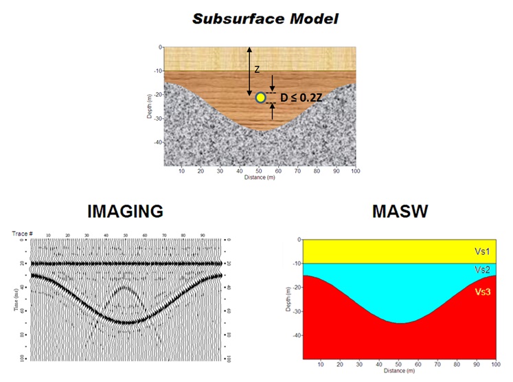
- Figure 1. Comparison of MASW as a characterization method and reflection as an imaging method by using a subsurface model
consisting of layers and a small-size anomaly (void).
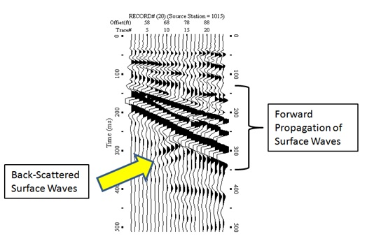
- Figure 2. A field record acquired over a shallow tunnel at about 2-m depth that shows back-scattered surface waves from the
tunnel as well as forward propagation of surface waves.
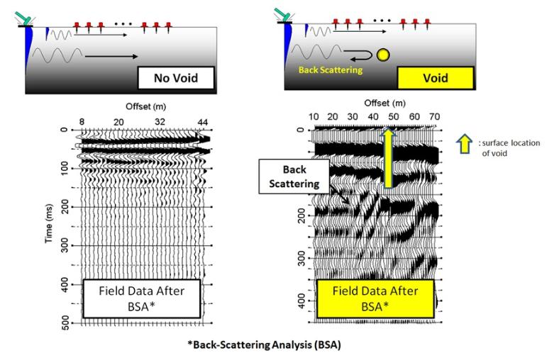
- Figure 3. Schematic illustrating how back-scattered surface waves are generated (top) and two back-scattering-analysis (BSA)
sections analyzed from two sets of real data.
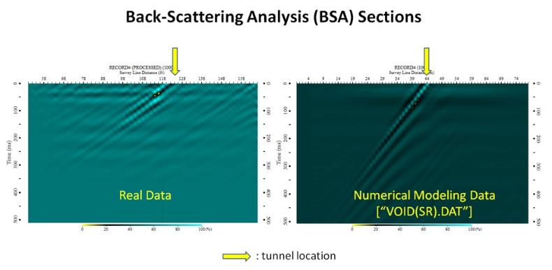
- Figure 4. Two sets of back-scattering-analysis (BSA) sections analyzed from real and model data sets that show the features
originating from the exact known surface locations; 124-ft for the real data and 44-m for the model data.
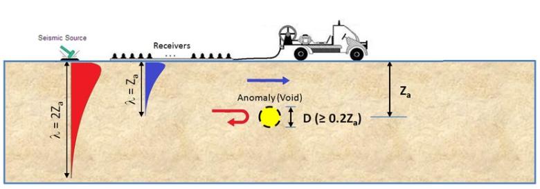
- Figure 5. A schematic illustrating that the penetration depth of surface waves is about one wavelength in which most of the energy
(~99%) is confined (illustrated by the amplitude variation with depth). It also illustrates that the back-scattering occurs only for those
surface waves penetrating deeper than the anomaly (void).
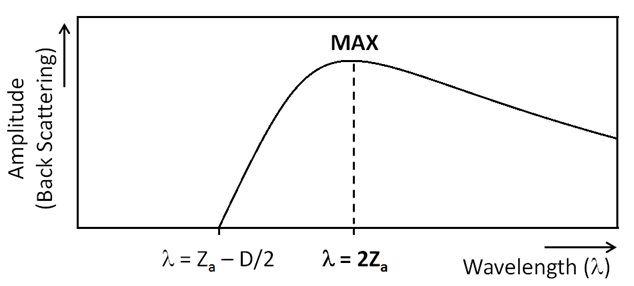
- Figure 6. A conceptual graph that shows how the amplitude of the back-scattered surface waves changes with wavelength (Lamda)
once it becomes longer than the depth to the top of the anomaly. Then, the maximum amplitude occurs when it becomes
approximately twice the anomaly depth (Lamda=2Za).
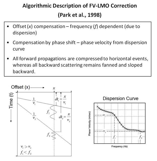
- Figure 7. Algorithmic description of the linear-move-out (LMO) correction used in Park et al. (1998).
Park Seismic LLC, Shelton, Connecticut, Tel: 347-860-1223, Fax: 203-513-2056, Email: parkseis@parkseismic.com
