
ParkSEIS© (PS) - Modeling Dispersion Curves
A (Rayleigh) dispersion curve consists of phase velocities at different frequencies that represent theoretically possible propagation modes of
(Rayleigh) surface waves. For a given frequency, there are multiple phase velocities at which surface waves can travel; the slowest velocity is called
the fundamental mode (M0), the next higher velocity is called the 1st higher mode (M1), the next higher one is called the 2nd higher mode (M2), and
so on. Collection of such phase velocities of the same mode is called the fundamental-mode (M0) dispersion curve, the first higher mode the (M1)
dispersion curve, and so on. In theory, the ultimate governing equation that predicts possible phase velocities at a given frequency is the elastic-
wave equation (Sheriff and Geldart, 1982). A derived formulation predicts that phase velocities are determined by solving a characteristic equation
(also called "dispersion function") of a layered-earth model that consists of shear-wave velocity (Vs), compressional-wave velocity (Vp), and density
(rho) parameters assigned to horizontally homogeneous layers of different thicknesses (h's). In practice, however, numerical approaches are taken
to find the closest values ("roots") to the theoretical solutions. According to Schwab and Knopoff (1972), roots to the dispersion function are
searched by continuously changing the possible phase velocity for a given frequency until the function becomes the opposite sign—a numerical
method called the bisection (Press et al., 1992).
This module of the ParkSEIS calculates Rayleigh-wave dispersion curves based on the FORTRAN IV program presented in Schwab and Knopoff
(1972). The input to this module is a layered-earth model (*.LYR) that can be obtained either as an output from the inversion of a measured
dispersion curve or as a separate model artificially created by using the "1-D Vs Profile" display module included in the main menu. In fact, this
(forward) modeling module is used in the inversion analysis that calculates the theoretical M0 dispersion curve from the velocity (Vs) model that is
continuously updated during the inversion process. Although the input file (*.LYR) includes attenuation parameters (Qs and Qp) for each layer, they
are not used during the dispersion-curve modeling and only the four aforementioned parameters (Vs, Vp, rho, and h) are used. Generation of an
accurate dispersion curve will depend on the way the bisection method searches for the root by continuously updating the testing phase velocity. A
smaller increment during the update procedure can increase the accuracy in the phase velocity as well as in modal identity (M0, M1, etc.), but at the
expense of longer computing time. This is controlled by a parameter called "Search integrity in phase velocity" included in the "Searching option"
tab. The default value (100) is determined through an extensive test with diverse layer models and therefore usually sufficient to achieve the highest
practical accuracy needed in most cases. However, the higher integrity (that will make the bisection interval smaller) can always be tested to
examine if different results are produced.
As far as the velocity (Vs) structure of the input layer model does not include the "inverse velocity" on top (i.e., Vs of top layer is higher than that of the
underlying layer), the modeled dispersion curves usually follow those dispersion trends observed in reality. However, with an inverse Vs structure
(for example, pavement or a stiff layer on the surface), the observed dispersion trend is determined not only by the trend of the fundamental mode
(M0) but also by a trend created from the mixture of successive higher modes for those frequencies where corresponding wavelengths (Lamda's)
become comparable to the thickness (h) of the top layer (e.g., Lamda ≤ 6h). This "mixed" dispersion trend is often referred as the "apparent"
dispersion curve (AM0). The transition from one mode to next ("mode jump") usually occurs at the point where the two curves get closest to each
other in phase velocity while searching from the low-frequency end (Figure 1). This is the way the modeling algorithm generates the apparent
dispersion curve ["*(AM0).dc"] under such an inverse velocity structure by calculating two successive modes of dispersion curves and searching for
the proximity point. Generation of an AM0 curve takes significantly longer computing time because of the necessity to calculate multiple modes. The
calculation of an AM0 curve becomes challenging at such high frequencies where wavelengths become close to the thickness of the top layer itself.
This is because of the theoretical limit that Rayleigh waves can exist only at phase velocities slower than the velocity (Vs) of the half space (Thrower,
1965). Higher mode calculation in this frequency (wavelength) range becomes less accurate and the calculated AM0 curve starts to deviate from the
real trend observed (Figure 2). Ryden et al. (2004) indicated that the accurate calculation of higher modes should include the dispersion function
solutions in complex-number domain (instead of the real number) that take significantly longer computing time. In addition, a separate calculation
of the excitability function should also be accompanied in order to determine the realistic trend for the AM0 curve. These reasons make it impractical
to include the complex-domain approach as a routine approach. On the other hand, Martincek (1994) verified that the AM0 trend can be replaced
with a sufficient accuracy by the fundamental-mode asymmetric Lamb-wave dispersion curve (A0) (Ryden et al., 2003) for high frequencies where
corresponding wavelengths become shorter than six to seven times the thickness of the top layer (i.e., Lamda ≤ 6h-7h) (Figure 2). Therefore,
choosing the "Apply Lamb approx. at high-frequency end" option is recommended whenever the calculated AM0 curve shows erratic patterns. The
"Apply Lamb approx. at high-frequency end" option is included in the "Inverse velocity (Vs)" tab.
- See user guide.
A (Rayleigh) dispersion curve consists of phase velocities at different frequencies that represent theoretically possible propagation modes of
(Rayleigh) surface waves. For a given frequency, there are multiple phase velocities at which surface waves can travel; the slowest velocity is called
the fundamental mode (M0), the next higher velocity is called the 1st higher mode (M1), the next higher one is called the 2nd higher mode (M2), and
so on. Collection of such phase velocities of the same mode is called the fundamental-mode (M0) dispersion curve, the first higher mode the (M1)
dispersion curve, and so on. In theory, the ultimate governing equation that predicts possible phase velocities at a given frequency is the elastic-
wave equation (Sheriff and Geldart, 1982). A derived formulation predicts that phase velocities are determined by solving a characteristic equation
(also called "dispersion function") of a layered-earth model that consists of shear-wave velocity (Vs), compressional-wave velocity (Vp), and density
(rho) parameters assigned to horizontally homogeneous layers of different thicknesses (h's). In practice, however, numerical approaches are taken
to find the closest values ("roots") to the theoretical solutions. According to Schwab and Knopoff (1972), roots to the dispersion function are
searched by continuously changing the possible phase velocity for a given frequency until the function becomes the opposite sign—a numerical
method called the bisection (Press et al., 1992).
This module of the ParkSEIS calculates Rayleigh-wave dispersion curves based on the FORTRAN IV program presented in Schwab and Knopoff
(1972). The input to this module is a layered-earth model (*.LYR) that can be obtained either as an output from the inversion of a measured
dispersion curve or as a separate model artificially created by using the "1-D Vs Profile" display module included in the main menu. In fact, this
(forward) modeling module is used in the inversion analysis that calculates the theoretical M0 dispersion curve from the velocity (Vs) model that is
continuously updated during the inversion process. Although the input file (*.LYR) includes attenuation parameters (Qs and Qp) for each layer, they
are not used during the dispersion-curve modeling and only the four aforementioned parameters (Vs, Vp, rho, and h) are used. Generation of an
accurate dispersion curve will depend on the way the bisection method searches for the root by continuously updating the testing phase velocity. A
smaller increment during the update procedure can increase the accuracy in the phase velocity as well as in modal identity (M0, M1, etc.), but at the
expense of longer computing time. This is controlled by a parameter called "Search integrity in phase velocity" included in the "Searching option"
tab. The default value (100) is determined through an extensive test with diverse layer models and therefore usually sufficient to achieve the highest
practical accuracy needed in most cases. However, the higher integrity (that will make the bisection interval smaller) can always be tested to
examine if different results are produced.
As far as the velocity (Vs) structure of the input layer model does not include the "inverse velocity" on top (i.e., Vs of top layer is higher than that of the
underlying layer), the modeled dispersion curves usually follow those dispersion trends observed in reality. However, with an inverse Vs structure
(for example, pavement or a stiff layer on the surface), the observed dispersion trend is determined not only by the trend of the fundamental mode
(M0) but also by a trend created from the mixture of successive higher modes for those frequencies where corresponding wavelengths (Lamda's)
become comparable to the thickness (h) of the top layer (e.g., Lamda ≤ 6h). This "mixed" dispersion trend is often referred as the "apparent"
dispersion curve (AM0). The transition from one mode to next ("mode jump") usually occurs at the point where the two curves get closest to each
other in phase velocity while searching from the low-frequency end (Figure 1). This is the way the modeling algorithm generates the apparent
dispersion curve ["*(AM0).dc"] under such an inverse velocity structure by calculating two successive modes of dispersion curves and searching for
the proximity point. Generation of an AM0 curve takes significantly longer computing time because of the necessity to calculate multiple modes. The
calculation of an AM0 curve becomes challenging at such high frequencies where wavelengths become close to the thickness of the top layer itself.
This is because of the theoretical limit that Rayleigh waves can exist only at phase velocities slower than the velocity (Vs) of the half space (Thrower,
1965). Higher mode calculation in this frequency (wavelength) range becomes less accurate and the calculated AM0 curve starts to deviate from the
real trend observed (Figure 2). Ryden et al. (2004) indicated that the accurate calculation of higher modes should include the dispersion function
solutions in complex-number domain (instead of the real number) that take significantly longer computing time. In addition, a separate calculation
of the excitability function should also be accompanied in order to determine the realistic trend for the AM0 curve. These reasons make it impractical
to include the complex-domain approach as a routine approach. On the other hand, Martincek (1994) verified that the AM0 trend can be replaced
with a sufficient accuracy by the fundamental-mode asymmetric Lamb-wave dispersion curve (A0) (Ryden et al., 2003) for high frequencies where
corresponding wavelengths become shorter than six to seven times the thickness of the top layer (i.e., Lamda ≤ 6h-7h) (Figure 2). Therefore,
choosing the "Apply Lamb approx. at high-frequency end" option is recommended whenever the calculated AM0 curve shows erratic patterns. The
"Apply Lamb approx. at high-frequency end" option is included in the "Inverse velocity (Vs)" tab.
| |
| |
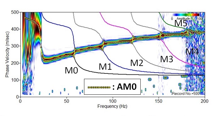
Figure 1. Dispersion image and modal dispersion curves (M0-M5) modeled from the velocity (Vs) model displayed in Figure 2a.
The dispersion image indicates that the actual observed dispersion trend follows the "apparent" dispersion curve (AM0) that is
created by continuous mode jumping between the two successive modes of curves at the place where they get closest to each
other.
The dispersion image indicates that the actual observed dispersion trend follows the "apparent" dispersion curve (AM0) that is
created by continuous mode jumping between the two successive modes of curves at the place where they get closest to each
other.
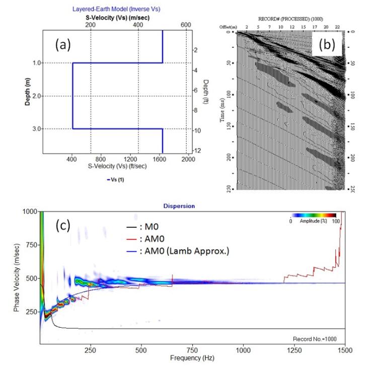
method. Corresponding dispersion image is displayed in (c) where the fundamental-mode (M0) and apparent (AM0) to
indicate that it can be a more accurate and reliable alternative at such frequencies where corresponding wavelengths come
close to the thickness of the top layer itself.
indicate that it can be a more accurate and reliable alternative at such frequencies where corresponding wavelengths come
close to the thickness of the top layer itself.
